Colocalization

To introduce spacedeconvs celltype colocalization and distribution analysis functions we will utilize a deconvolution result obtained from internal sample data and the deconvolution method EPIC. Note that EPIC requires unnormalized data and is building the signature and deconvoluting in one step. Therefore only deconvolute() is called.

library(spacedeconv)
library(SpatialExperiment)

data("single_cell_data_3")
data("spatial_data_3")

single_cell_data_3 <- spacedeconv::preprocess(single_cell_data_3)
spatial_data_3 <- spacedeconv::preprocess(spatial_data_3)

single_cell_data_3 <- spacedeconv::normalize(single_cell_data_3, method = "cpm")
spatial_data_3 <- spacedeconv::normalize(spatial_data_3, method = "cpm")

signature <- spacedeconv::build_model(
  single_cell_obj = single_cell_data_3,
  cell_type_col = "celltype_major",
  method = "dwls", verbose = T, dwls_method = "mast_optimized", ncores = 10
)

deconv <- spacedeconv::deconvolute(
  spatial_obj = spatial_data_3,
  single_cell_obj = single_cell_data_3,
  cell_type_col = "celltype_major",
  method = "dwls",
  signature = signature,
  assay_sp = "cpm"
)

Available colocalization functions

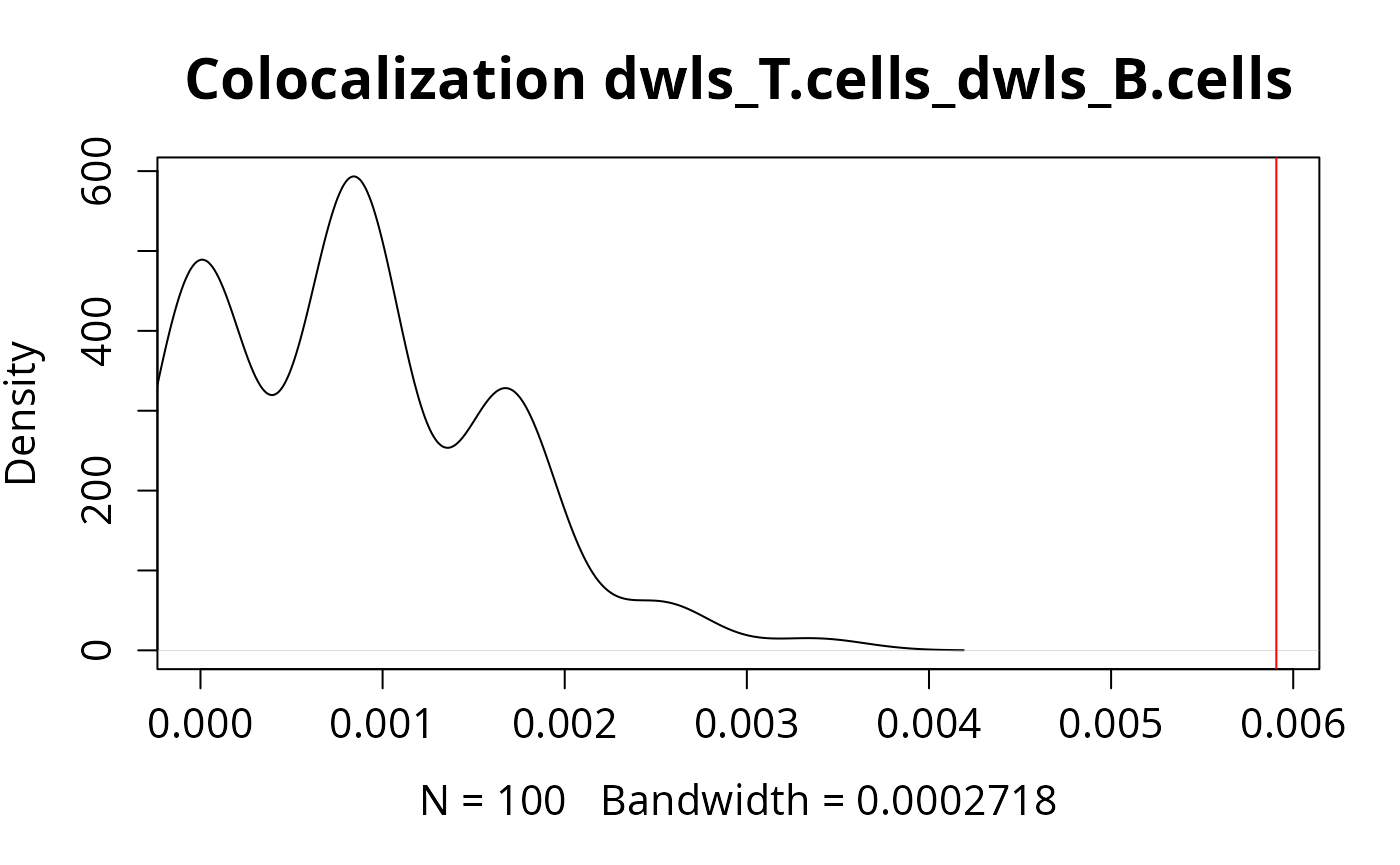
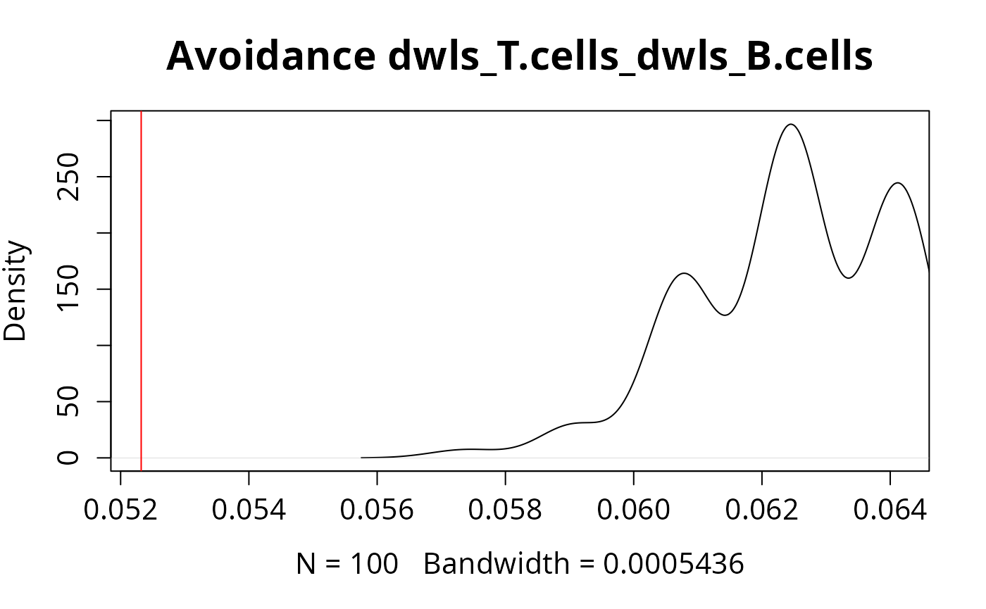
1. ‘cell_pair_localization()’ calculates colocalization and avoidance of two celltypes based on a random distribution.
2. ‘ripleys_k()’ calculates Ripley´s K statistic and outputs corresponding graph

1. ‘cell_pair_localization()’

Calculates colocalization and avoidance statistics of two celltypes of interest based on a random distribution. Internally, the presence or absence of the celltypes is determined based on the antimode of the celltype density distribution. Spotwise comparisons or groupwise comparisons with increasing distances are possible. Thereby, distance = 0 corresponds to a spotwise approach, distance = 1 considers hexagonal rings of spots around each spot and distance = 2 refers to two rings of spots around each spot.

spacedeconv::cell_pair_localization(deconv, method = "dwls", cell_type_A = "dwls_T.cells", cell_type_B = "dwls_B.cells", density = TRUE, distance = 0)
#> Calculating presence matrix...
#> [1] "Calculating Antimode cutoffs"
#> Warning in locmodes(logscore, mod0 = 2, display = F): If the density function
#> has an unbounded support, artificial modes may have been created in the tails

#> Warning in locmodes(logscore, mod0 = 2, display = F): If the density function
#> has an unbounded support, artificial modes may have been created in the tails

#> Warning in locmodes(logscore, mod0 = 2, display = F): If the density function
#> has an unbounded support, artificial modes may have been created in the tails

#> Warning in locmodes(logscore, mod0 = 2, display = F): If the density function
#> has an unbounded support, artificial modes may have been created in the tails

#> Warning in locmodes(logscore, mod0 = 2, display = F): If the density function
#> has an unbounded support, artificial modes may have been created in the tails

#> Warning in locmodes(logscore, mod0 = 2, display = F): If the density function
#> has an unbounded support, artificial modes may have been created in the tails

#> Warning in locmodes(logscore, mod0 = 2, display = F): If the density function
#> has an unbounded support, artificial modes may have been created in the tails

#> Warning in locmodes(logscore, mod0 = 2, display = F): If the density function
#> has an unbounded support, artificial modes may have been created in the tails

#> Warning in locmodes(logscore, mod0 = 2, display = F): If the density function
#> has an unbounded support, artificial modes may have been created in the tails

#>  coloc_real.coloc           coloc_p   coloc_rand_mean coloc_ratio.coloc 
#>              0.01              0.00              0.00              7.00 
#>  avoid_real.avoid           avoid_p   avoid_rand_mean avoid_ratio.avoid 
#>              0.05              1.00              0.06              0.84

2. ‘riples_k()’

Determines the spatial distribution of a celltype based on Ripley´s K function. A matrix with presence or absence values for each celltype, determined using the antimode of the celltype density distribution, is internally taken as input.

spacedeconv::ripleys_k(deconv, method = "dwls", cell_type = "dwls_B.cells")
#> [1] "Calculating Antimode cutoffs"
#> Warning in locmodes(logscore, mod0 = 2, display = F): If the density function
#> has an unbounded support, artificial modes may have been created in the tails

#> Warning in locmodes(logscore, mod0 = 2, display = F): If the density function
#> has an unbounded support, artificial modes may have been created in the tails

#> Warning in locmodes(logscore, mod0 = 2, display = F): If the density function
#> has an unbounded support, artificial modes may have been created in the tails

#> Warning in locmodes(logscore, mod0 = 2, display = F): If the density function
#> has an unbounded support, artificial modes may have been created in the tails

#> Warning in locmodes(logscore, mod0 = 2, display = F): If the density function
#> has an unbounded support, artificial modes may have been created in the tails

#> Warning in locmodes(logscore, mod0 = 2, display = F): If the density function
#> has an unbounded support, artificial modes may have been created in the tails

#> Warning in locmodes(logscore, mod0 = 2, display = F): If the density function
#> has an unbounded support, artificial modes may have been created in the tails

#> Warning in locmodes(logscore, mod0 = 2, display = F): If the density function
#> has an unbounded support, artificial modes may have been created in the tails

#> Warning in locmodes(logscore, mod0 = 2, display = F): If the density function
#> has an unbounded support, artificial modes may have been created in the tails
#> Function value object (class 'fv')
#> for the function r -> "K"["TRUE","TRUE"](r)
#> ................................................................................
#>      Math.label                        
#> r    r                                 
#> theo {K[list(TRUE,TRUE)]^{pois}}(r)    
#> iso  {hat(K)[list(TRUE,TRUE)]^{iso}}(r)
#>      Description                                          
#> r    distance argument r                                  
#> theo theoretical Poisson "K"["TRUE","TRUE"](r)            
#> iso  isotropic-corrected estimate of "K"["TRUE","TRUE"](r)
#> ................................................................................
#> Default plot formula:  .~r
#> where "." stands for 'iso', 'theo'
#> Recommended range of argument r: [0, 1338.8]
#> Available range of argument r: [0, 1338.8]